

3 Excel Hacks that Save Lives
Since I started working in digital, Excel has become my best friend.
Excel is a war machine. But a machine that must be fed to work properly. I learned to tame the beast over the years so well that now I would not know how to work without it.
I wanted to give you three of my most useful tips, the ones that I use concretely and regularly.
How to extract the time in a date?
When you upload the posts statistics from Facebook, you get a date format that looks like this.
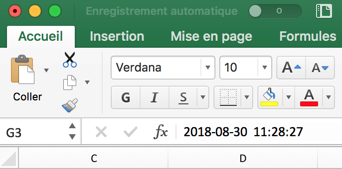
In the same cell, we have the date AND time of post. This creates a slight issue when you want to use this data to know, for example, at what time to post to have a higher probability of obtaining likes.
Over time, I have found a very simple formula that solves this issue in no time at all. Here’s the secret:
Insert two new columns on the right, which you will name “Date only” and “Time only”.
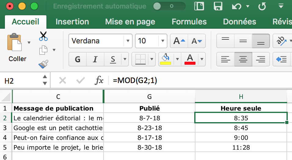
For “Time Only”
- Enter the formula =MOD([your complete date cell];1)
- Assign the Time Format to the “Time Only” column.
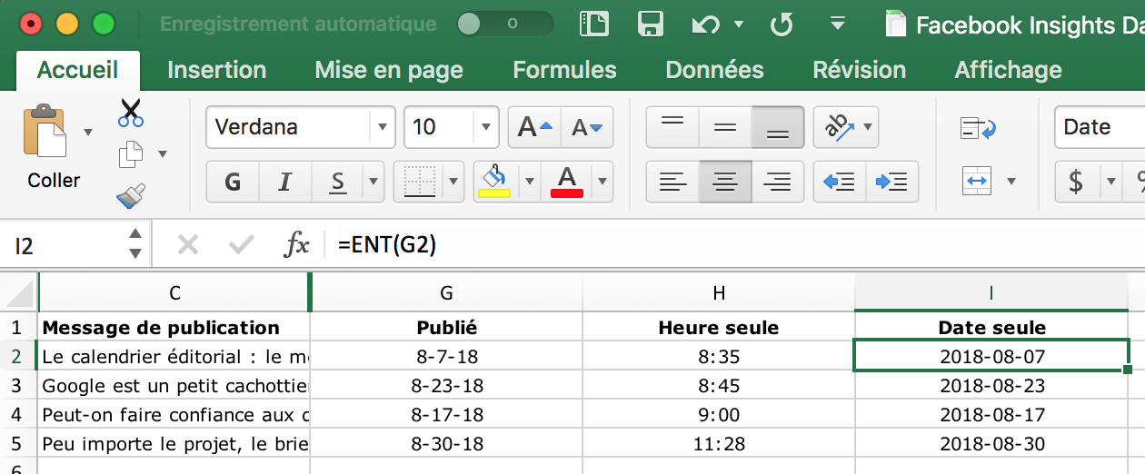
For “Date only”
- Enter the formula =ENT([your complete date cell])
- Assign the Date Format to the “Time Only” column.
TADAM! Now, all you have to do is analyze.
How to rename a range of cells?
Is that possible? Yes it is. And you have no idea how often that serves me.
Let’s say I make a chart for myself to evaluate the performance of my posts. There are some data ranges that I will often need, such as the reach or the number of clicks for example. Instead of wasting time searching each time for which cell range to refer to, I assign it a custom name from the beginning and then always refer to it. It makes the formulas more digestible and understandable.
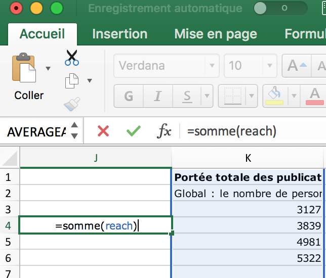
There is a “Name Zone” in Excel. To use it, simply select the cell range (or a column or an entire row for example) and enter the desired name in the name field.
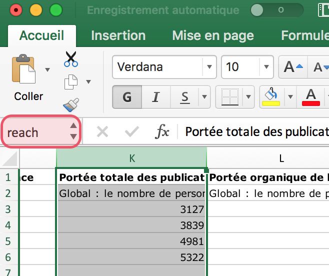
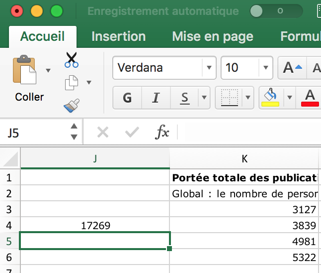
Whenever you want to refer to this cell range in your formulas, all you have to do is enter the given name (like to find the reach sum in my example).
How to manage the display by data level?
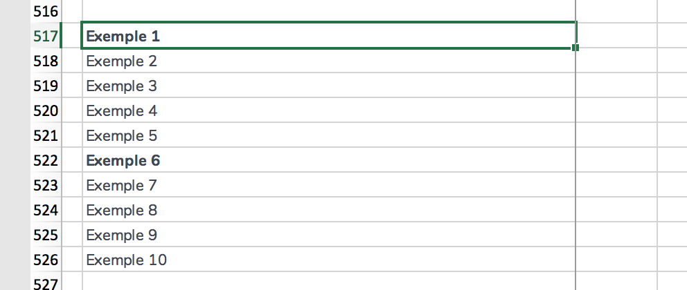
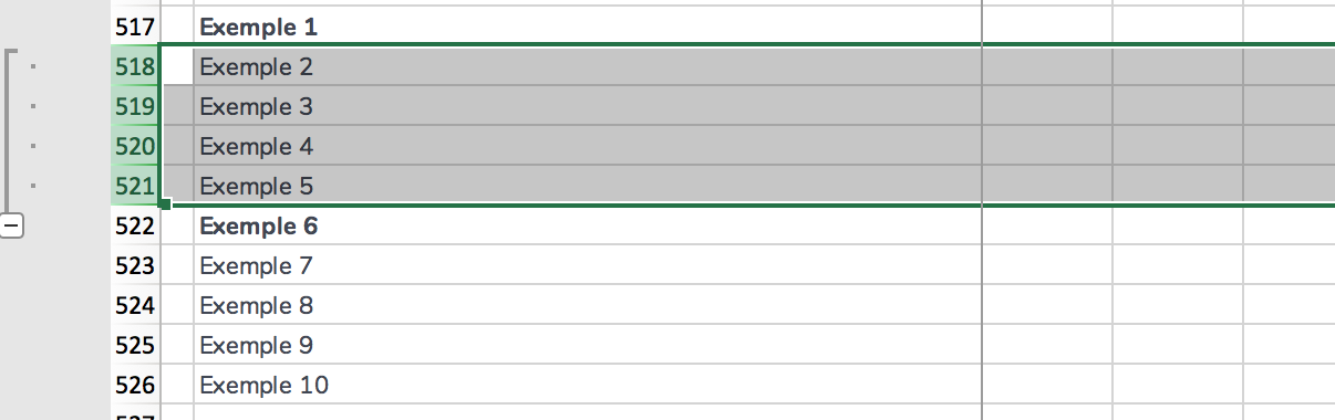
I recently had a display puzzle to solve on Excel. I wanted to create a double entry table to clarify the roles and responsibilities of my project teams. I was looking for a way to add a “little plus” or a “little minus” next to my cell ranges to have different levels of reading: from the most general to the most micro, depending on what you are looking for in terms of information.
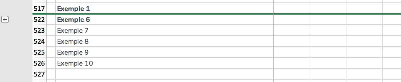
So I wanted to easily hide or show data groups. And… I couldn’t remember what the function was called to ask Google for help! Fortunately, it was finally super simple. I only had to use the “Group” function.
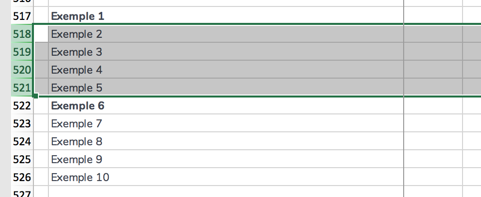
Select the data to be grouped, and then under the Data tab, in the Plan group, click Group, click Lines, then click OK.
It’s simple, isn’t it? I swear to you: it’s a game change!

It’s really worth doing it in more complex files or ones that are used as templates.
Try it and give me some news!

📞 514-844-1050 📧 bianka@vionumerique.com